Excel Tutorial: INDEX MATCH primer
Two weeks, we looked at the syntax of VLOOKUP, INDEX and MATCH. Last weeks tutorial should have walked you through the basics of VLOOKUP. In this post, we’ll use a similar file from the VLOOKUP tutorial to find a value from the table using INDEX and MATCH.
If you haven’t had a chance yet, please go through the VLOOKUP tutorial. Alternatively, if you’re ready to jump right into INDEX/MATCH, then let’s get started.
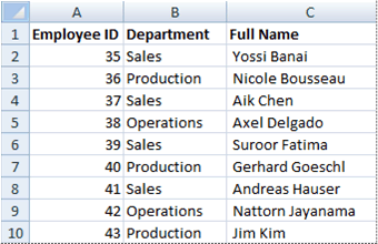
Firstly, create the above table in Excel. I’ll be using Excel 2010 in my example. You can also download the examples file before you proceed. The file contains a Questions sheet which you can practice in and a Solutions sheet with the answers.
If you haven’t had a chance to review the basic syntax of the functions, please do read this post before you continue.
Step 1: Basic usage by hard-coding row_num and column_num
The screenshot below gives you the formula to use
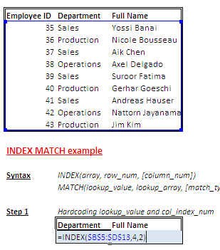
As you can see this is very basic. All you have to do is pass the value of the array as the first parameter and row number and column number you want to look up. In this example, it will fetch “Operations” which is the value of cell sitting in the 4th row and 2nd column, i.e. corresponding to 38.
To pull the full name, you will use =INDEX($B$5:$D$13,4,3).
Step 2: Cell-referenced row_num (using MATCH) and hardcoded column_num
Using INDEX in the above method is not useful at all, since it is not efficient to try passing the row numbers, which beats the entire concept of “looking up”.
The screenshot below shows you how you can get around this by using MATCH in combination with INDEX.

In this example instead of the number 4 we use MATCH($B27,$B$5:$B$13,0). This will search out the Employee ID (38) from the array ($B$5:$B$13) and check for an exact match. In this example, it returns the number 4, which is what we want.
Step 3: Cell-referenced row_num (using MATCH) and cell-referenced column_num
This is similar to our VLOOKUP example.

Instead of the column_num being stated as 3, we use a cell reference (D$31) to pass the column number
Step 4: Cell-referenced row_num and column_num using MATCH
Let’s take this up a notch. The real power of INDEX is to use MATCH for both the row and column numbers. Check out the screenshot below which gives you the formula you need to use.

The second MATCH will search through the header array ($B$4:$D$4) and return the column number. This makes your table completely dynamic.
Note that it is more efficient to have the column numbers separately pulled up if you’re using more than one row, since this ensures cleaner formulae. You can see the solution for this in the excel file you can download from the end of this post.

Concluding words
I hope the above set of examples gives you a good introduction to using INDEX in combination with MATCH. I had mentioned in last week’s post that VLOOKUP has a limitation that the data that you want to match has to be present in the first column of the array. In our example above, this is the Employee ID.
INDEX and MATCH allow you to overcome this limitation, since you have complete freedom to pass any array to the MATCH. e.g. check out the screenshot below (Step 6 in our examples file).

Ultimately, it is a matter of choice on whether to use VLOOKUP or INDEX-MATCH. I prefer using VLOOKUP as my first option since it is much easier to use and results in a much cleaner formula. However, when I don’t have data in the first column I use INDEX in combination with MATCH.
If you have any questions regarding INDEX and MATCH, leave a comment below and I’ll try to answer it. You can also try Stack Overflow which gives you access to a much larger community of users.
Downloads
Download “INDEX MATCH examples”
INDEX-MATCH-examples.zip – Downloaded 2216 times – 10.92 KB
