Data Tables is also an advanced topic in Microsoft Excel that falls under the category of What-If Analysis. What-If or Sensitivity Analysis is carried out to study the variation of the output to changes in the input variable. Data Tables are an extremely powerful tool when used carefully. They give you insight on outputs for a varying level of inputs. In this post, I’ll explain to you how a single variable data table can be created via an example. I’ll be using Microsoft Excel 365 but this tutorial will also apply to older versions of Excel.
Excel Help describes a data table as:
A data table is a range of cells that shows how changing one or two variables in your formulas (formula: A sequence of values, cell references, names, functions, or operators in a cell that together produce a new value. A formula always begins with an equal sign (=).) will affect the results of those formulas. Data tables provide a shortcut for calculating multiple results in one operation and a way to view and compare the results of all the different variations together on your worksheet.
Defining the problem
Consider a case of compound interest, where you invest a certain amount of money in a bank deposit and the amount is compounded every year.
Formula for calculating compound interest:
A = P * (1 + r/n) ^ nt
Where:
P = principal amount (initial investment)
r = annual interest rate (as a decimal)
n = number of times the interest is compounded per year
t = number of years
A = amount after time t
Now, if suppose we want to see what the final amount will be at different interests rates, we can use a data table.
The solution
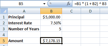
Open a new excel file and enter the following as given in the screenshot below:
The cell B5 has the formula =B1*(1+B2)^B3
As you can see, the $5,000 invested at 7.5% for 5 years will give $7,178.15.
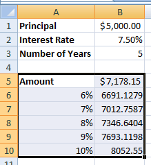
Now, we will create a data table to see what amount we will receive by changing the interest rate.
Fill cells A6 to A10 with different interest rates. I’ve filled it with values from 6% to 10%. Now, select the cells A5:B10.
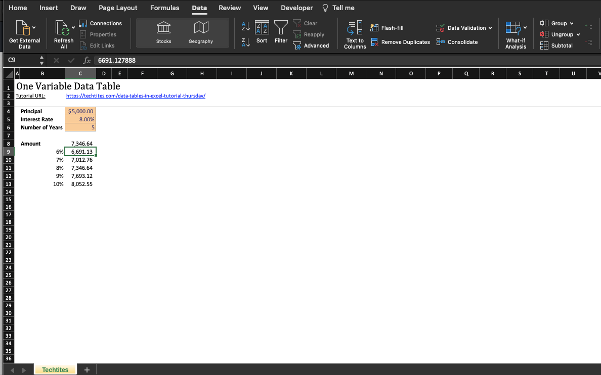
In Excel, navigate to Data > What-If Analysis > Data Table. You can use the shortcut key Alt + D + T in this order in Windows.
This will popup a window where you will be asked to enter Row Input Cell and the Column Input Cell. Select the Column Input Cell as $B$2 and leave the Row Input Cell blank and hit OK.
The values will be filled in as shown below. You can choose to format them as currency, but that I have left it up to you.
How it works?
Well, we did get the results, but the question remains on what just happened.
To understand this simply, the Column Input Cell is the variable whose value we are going to vary. If supposing the data was presented horizontally instead of vertically which is our case, then you would need to select it as a Row Input Cell.
The values in cells A6 to A10 are then passed to the formula in cell B5 and the corresponding results are populated in cells B6 to B10.
If you look at cells B6 to B10, they contain the formula {=TABLE(,B2)}
Can you try creating a Data Table using a Row Input Cell? Why don’t you post your solution below or on your blog and post a link below in the comments area.
We created a One Variable Data Table. The next step is learning how to create a Two Variable Data Table.
thanks for? the tutorial I tried to place the row / column input cell in a another sheet, it did not work. is it possible at all to work this tool when the row / column input cell in another sheet ? thanks again itzik
We use cookies to ensure that we give you the best experience on our website. If you continue to use this site we will assume that you are happy with it.OkPrivacy policy


thanks for? the tutorial
I tried to place the row / column input cell in a another sheet, it did not work.
is it possible at all to work this tool when the row / column input cell in another sheet ?
thanks again
itzik
No you can’t. All inputs need to be in the same sheet.