Excel Tutorial: SUMIF with Multiple Conditions
The title of the post is a bit of a misnomer because the SUMIF function in Excel does not allow you to have more than condition.
Excel 2007 introduced the SUMIFS function which allowed for multiple conditions. However, if you are using any version prior to Excel 2007 or if the persons who will be using your Excel workbook will be using a version prior to Excel 2007, then the SUMIF function will throw up an error.
That is a problem a colleague faced at work. To solve this problem you can use SUMPRODUCT along with double negation. The double negation is simply two minus signs one after an another. The net effect is that it doesn’t change the value of the calculations.
The reason we use the double negation is because, Excel does not always understand that TRUE=1 and FALSE=0 when you use SUM or SUMPRODUCT.
Using SUMIFS

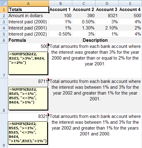
Let’s take a look at Example 2 on the SUMIFS
The screenshot is pretty self explanatory. I’ve added an additional line to demonstrate the use of four conditions with SUMIFS. The code that you will need to put in cell A9 is =SUMIFS(B2:E2, B5:E5, ">=1%", B5:E5, "<=3%", B4:E4, ">1%",B3:E3,">1%")
Using SUMPRODUCT
Now, we will use SUMPRODUCT for the same.
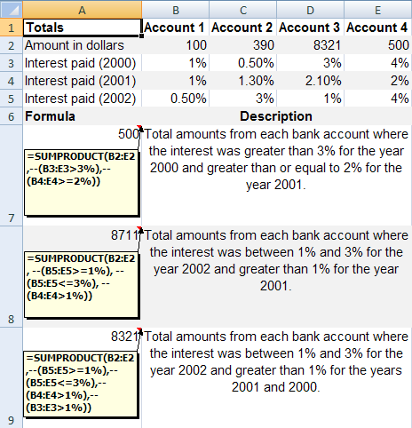
I’ve put the functions in the cell as a comment. Let’s take a look at the function in cell A7. It is =SUMPRODUCT(B2:E2,--(B3:E3>3%),--(B4:E4>=2%))
The syntax for SUMPRODUCT is =SUMPRODUCT(array1,array2,array3, ...). Comparing with our code above,
- array1 = B2:E2 – This is the array from whom
- array2 = –(B3:E3>3%) – This is the first condition
- array3 = –(B4:E4>=2%) – This is the second condition
Breaking down --(B3:E3>3%), the first calculation step is to evaluate (B3:E3>3%). This results in an array {FALSE, FALSE, FALSE, TRUE}.
Next, the first minus converts this into numerics. The resultant array is {0,0,0,-1} and the second negation converts the array into {0,0,0,1}. Similarly, array3 evaluates to {0,0,1,1}.
The SUMPRODUCT then kicks in as: 100*0*0 + 390*0*0 + 8321*0*1 + 500*1*1 = 500
You can study the remaining two examples.
One point that needs to be noted is that “the array arguments must have the same dimensions. If they do not, SUMPRODUCT returns the #VALUE! error value.”
A workaround to this is to include dummy cells having 0 values to pad the arrays which are of a smaller dimension.
Did you like this Tutorial? Would you like to see more Excel tips / tutorials? Please do comment below. If you have something to share please do write in.
Download “SUMPRODUCT, SUMIFS and SUMIF example”
SUMPRODUCT_SUMIFS.zip – Downloaded 3604 times – 10.22 KB




thank you very much. resolved my problem. excellent job.
Thanks a lot. My search is over.
Thank you guys, very useful indeed.
Aled
Do you want to read about the syntax and usage of an Excel 2013 or VBA function in your native language and practice with a demo workbook ?
The facts:
There are over 600 Excel & VBA functions in Office 2013.
Excel functions have been translated in 16 languages.
Microsoft offers over 20,000+ function help webpages in 50+ languages.
How to navigate fast among so many help pages ?
This free Ribbon Add-in will help you navigate to Microsoft’s online help pages with embedded workbooks, which can be downloaded to your computer for function inspection and in-depth practice.
http://www.spreadsheet1.com/excel-2013-translated-functions-free-addins.html