Two Variable Data Tables in Microsoft Excel Tutorial

In my last post, I taught you how to create a Single Variable Data Tables in Excel. As promised, in this tutorial I will cover creating a two variables data table. This allows you to flex two different variables simultaneously to see the output.

This tutorial assumes that you are comfortable with creating a single variable data table.

We’ll once again be looking at our Compound Interest example where you will be calculate what the amount you will receive at a certain interest rate after a specific period of time. You can also skip to the bottom of this post to download the example.

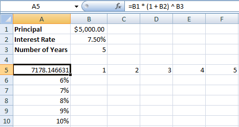
Create a new excel file and lay it out as shown in the screenshot above. Alternatively, you can start with the excel file from our previous example. In cell A5, enter the formula =B1*(1+B2)^B3.

As you can see, the $5,000 invested at 7.5% for 5 years will give $7,178.15.

A reminder of the formula for calculating compound interest:

A = P * (1 + r/n) ^ nt

Where:

• P = principal amount (initial investment)
• r = annual interest rate (as a decimal)
• n = number of times the interest is compounded per year
• t = number of years
• A = amount after time t

We will be varying the annual interest rate and the number of years to find the varying results.

After you have created the file according to the screenshot above, select the data range A5:F10.

In Excel, go to Data > What-If Analysis > Data Table or you can use the shortcut key Alt + D + T in this order in Windows.

This will popup a window where you will be asked to enter Row Input Cell and the Column Input Cell. Select the Column Input Cell as $B$2 and the Row Input Cell as $B$3 and hit OK.

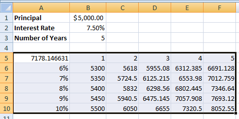
The cells will be populated as shown in the screenshot below. As usual, you can choose to format the same currency.

How does it work?

Cells B6:F10 hold the formula {=TABLE(B3,B2)}.

Here, the values B4 to F4 are substituted for B3 in the formula in cell A5 and values A6 to A10 are substituted for B2 in the formula in cell A5 and the results are then populated accordingly.

Hence, for 1 year at 8%, the amount is $5,400, for 3 years at 10%, the amount is $6,655.00 and so on.

You can download the sample XLSX file for your reference.